The Malaysian Election 2018

The 14thGeneral Election in Malaysia was held, with the unexpected victory of a coalition of opposition parties under the leadership ofDr Mahatir Mohamad, who previously served as Prime Minister between 1981 and 2003.

Among his first orders of business will be to spring his former deputy Prime Minister, Anwar Ibrahim, from jail and arrange him a pardon.  This will then allow Mahatir to pass the leadership on to Anwar.  Anwar’s wife will serve as deputy.

There has been much confusion in Malaysia over the process of transferring power.  This is a result of a lack of familiarity with the mechanics of a change in leadership.  This election represents the first change in government in Malaysia in over 60 years.

Mahatir achieved this victory despite the circumstances of the election being extremely favourable to the outgoing Prime Minister, Najib Razak.  These included:

  • A new ‘fake news’ law which could be used to prevent discussion of any sensitive topics.
  • The election being held mid-week when it would be more difficult for voters to attend polling places, potentially limiting the ability of Mahatir to attract voters.
  • A compliant press, with major print and broadcasting under government control.
  • A redistribution of electorates which was favourable to the incumbent government.
  • The fact that Mahatir paved the way for many of the practices which Najib continued.Jailing political opponents, limiting free speech and freedom of the press, were all practiced under Mahatir’s first tenure as Prime Minister.

Overwhelming these advantages, however, were:

  • A general dislike of Najib, due to his opulent lifestyle and questions about billions of dollars being routed to his personal accounts, which were never satisfactorily explained. Although understanding the nature of the international finance was difficult, Mahatir had an ability to bring this down to a simple, resonating message.
  • The respect with which Mahatir is held in Malaysia. This has in a sense inoculated him from attacks by the government and allowed him to get away with actions that no other opposition leader could, suh as leading mass protest marches.
  • Economic pressures – particularly the cost of living pressures.

The financial impact of the election result has seen the value of the Malaysian Ringgit fall and the price of companies exposed to Malaysian economy also fall on other stock markets.  The two days following the election were announced as public holidays when it became clear that the government would change, limiting impact on the Kuala Lumpur Stock Exchange.  I believe that there are a number of reasons for this fall:

  • Some economically popular, but potentially fiscally unwise items in the new Government’s platform – such as eliminating the 6% GST in Malaysia, which was introduced in 2015, and subsidising fuel. Anwar seems to be a centre-left politician, but friendly towards the West.
  • The uncertainty surrounding a new government in a country which has never seen a government of any party other than Barisan National.
  • The unexpected nature of the result.
  • The change in government redefining the relationship with the government and private sector. What were lucrative positions may now become potential headaches for firms as inevitable investigations into the previous governments’ activities highlight and punish corruption.  Less seriously, parties to ‘pet projects’ such as high-speed rail may be facing uncertainty. Anwar’s previous term as deputy prime minister saw him cut government spending, particularly in such projects.

Regardless of the success or otherwise of Malaysia’s new Government, it will provide an important service for years to come.  It will show Malaysians that they can change the government.

The Australian Federal Budget 2018-19

This is a budget that is seeking relying heavily on a dramatic uptick in business activity to support a reduced deficit, cuts in income tax and consistent real reduction in expenditure. This business activity is expected to be driven by continued solid investment in the non-mining sector and growth in the mining sector.

Figure 1: Investment Growth

The Economic Environment

The charts in Figure 1 highlight how similar the economic outlook is compared with last year’s budget.

  • GDP growth and CPI growth remain in line with the previous forecasts.
  • Unemployment marginally lower, (by around 0.25%).
  • Lower wage growth.

The personal income tax cut, highlighted by the Government, indicate that the government is seeking to achieve lower unemployment by providing an increasing share of workers disposable income.

Figure 2: Key Economic Statistics, Budgets 2018-19 v 2017-18


The global economy is expected to remain relatively unchanged compared with previous year’s budget, with the notable changes being stronger growth in Japan and US. While the budget does mention “recent tariff announcements by the US Administration, and fears that they may escalate, present uncertainties for both the US and global outlook”, this does not appear to be reflected in the numbers.

Personal income tax cuts

The key points about the personal income tax is that it will be introduced in stages, with lower income taxpayers being at the front of the queue as the cuts are rolled out over the coming years. The government has focussed on these tax cuts, restructuring their argument and allowing the corporate tax cuts which have commandeered so much political capital recently.

Excel Current Affairs: Today() and Now()

Microsoft Excel offers two common functions to refer to the current date and/or time: Today() and Now().

This short note describes the risks associated with the use of these functions and suggests that they be used with care.

Firstly, both of these functions are volatile. To understand why this is bad, we need a brief diversion into the way spreadsheets work. Excel maintains a list of cells which are impacted by changes in each cells value. In a simple financial model, changing the price may change revenue and profit lines, but seeing no link, Excel will not seek to recalculate the expense section of your workbook. This saves time. However, introducing volatile functions means that the spreadsheet will now recalculate these functions. Any cells which may rely on them. This will slow down your spreadsheet.

Secondly, and most importantly, these functions can be misleading if used in the way they are meant to be used. For example, a spreadsheet which generates a daily report could save the user time by using the TODAY() function – no need to update the day every day. However, this will then create issues unless it is based on a lookup of the date. Static numbers or formulae will lead to confusion.


Updated

The date look up table was imagining a report which looked up a figure from a daily time series.  In that case, the entire report will update with the latest day’s data, potentially being useful.  I was discouraging the attempt to have yesterday’s report being rendered confusing because the headings are now for today but it still holds yesterday’s results.


Australian Federal Budget Review 2017-18

Key Points

  • The budget outcome in 2017-18 is expected to be a deficit of $29.4b in cash terms
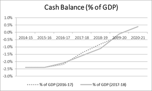
  • The 2017-18 Federal Budget forecasts a return to a small surplus ($7b or 0.4% of GDP) in 2020-21, with a budget deficit of $29.4b.
  • This is without any expected sharp reduction in expenditure which has been a feature of previous returns to surplus.
  • The political environment will act as a constraint on the Government’s ability to return the budget to surplus in the timetable outlined.

The Budget Result

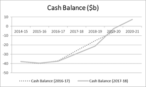
The budget outcome in 2017-18 is expected to be a deficit of $29.4b in cash terms. This compares with:

  • Previous year’s budget deficit of $37.6b
  • The forecast of $26.1b in the 2016-17 budget.

While the deficit has fallen this year, it is higher than what was expected. In the context of fiscal management, it is behind where we were expecting it to be in terms of a return to surplus. However, the government is continuing to forecast a return to surplus in 2020-21.

In recent years, the way that fiscal policy has been reported has changed – the focus is no longer on the size of that year’s surplus or deficit, but on the long-term outcome – when the budget will return to surplus. This budget confirms what was promised in last year’s budget, but was outside the projection period and forecasts a small deficit ($2.5b) in 2019-20, and a return to surplus in 2020-21.

Figure 1: Budget Outcome


A comparison with last year’s budget shows that the deficits 2018-19 deficit is expected to be higher (that is, expenditure exceeding receipts by a greater margin), and roughly in line in 2019-20.

It should be noted that this is in the context of an economic environment which is no better than, and arguably weaker than, that envisaged in the 2016-17 budget. This is discussed in more detail below.

When we take a longer-term view, as in Figure 2, we can see that since 1970-71, the budget has returned to surplus on three occasions:

  • 1981-82 for one year;
  • 1987-88 through 1989-90; and
  • 1997-98, following which it remained in surplus until 2008-09, with the exception of the year 2001-02.

Figure 2: Long term budget overview

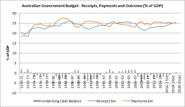
It can be seen that each of these returns to surplus was accompanies by significant reductions in expenditure (or payments). If the forecasts in this Budget hold, this will be the first budget in 50 years to return to surplus without a significant reduction in Government expenditure in GDP terms.

The Economic Environment

As mentioned above, the improvements in the long-term budget outlook (from 2019-20 on) discussed above is in contrast to a generally weaker economic environment.


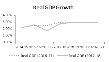
After achieving lower than expected economic growth in 2016-17, as shown in Figure 3, the forecasts in this budget revise the forecast GDP growth figures downwards until 2018-19. While this is reflected in the higher budget deficits in 2018-19.

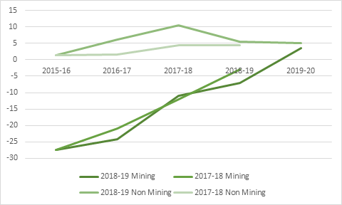
Figure 3: Real GDP Growth

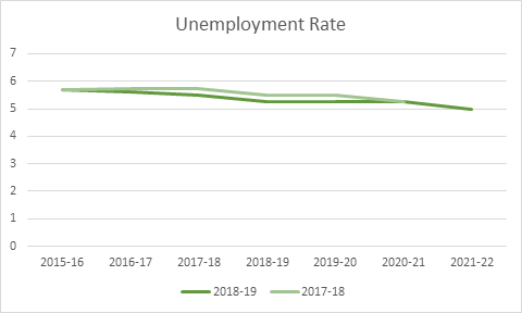
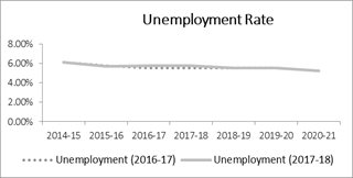
Unemployment forecasts (see Figure 3) remain relatively unchanged in this years budget compared with last year’s, with the slow, steady reduction in the unemployment rate repeated.

However, there unemployment rate in 2016-17 and 2017-18 is forecast to be 0.25 percentage points higher than those in last year’s budget.

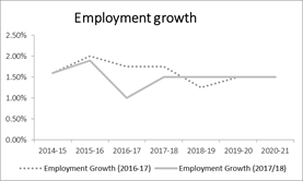
When examined with the GDP growth assumptions in the budget, it can ve seen that from 2018-19 through 2020-21 feature cumulatively lower employment growth (meaning that the stock of labour available is lower) and constant GDP growth. This carries an implicit assumption about either an increase in the productivity of the Australian labour force or a change in the way that labour is allocated away from less efficient sectors.

Figure 4: Employment and Unemployment forecasts


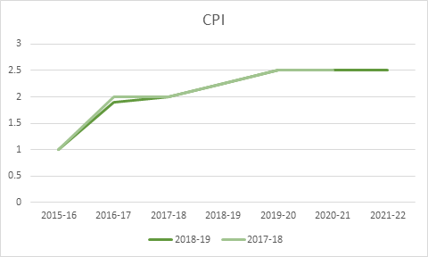
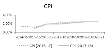
Inflation is forecast to remain at or below the middle of the RBA’s 2-3% comfort zone, suggesting little appetite for the central bank to increase Australia’s official interest rate. While this is a positive, such low inflation is typically associated with subdued economic growth. In relation to the Government’s previous budget, we note that inflation is expected to be lower than previously forecast.

Figure 5: CPI Outlook 2016-17 Budget -v- 2017-18 Budget


The Political Environment


In the absence of a strong economic outlook, the government will be required to finance the return to surplus through political capital. The increases in revenue which are designed to drive the return to surplus will be opposed by those who will face higher taxes, who it is assumed will be prepared to

However, there are limits on the Governments political capital, including:

  • A one seat majority in the House of Representatives;
  • Reliance on a diverse Senate, where it is required to negotiate with a range of minor parties with divergent interests and priorities;
  • The Government and Prime Minister’s continued unpopularity;
  • Competing, and even contradictory goals – measures which avoid short term hits to popularity are likely to impede the return to surplus which is increasingly being seen as a yardstick of economic management credentials.

Housing Affordability

In the period leading up to the budget, expectations were built around policies designed to improve housing affordability.

In broad terms, housing affordability is a difficult subject to address.

  • Australian house sizes have been increasing – making like for like assumptions difficult. How does a 3 bedroom, 2 bathroom house common in the 1970’s compare with a 5 bedroom, 3 bathroom today?
  • News stories featuring a charmless house achieving astronomical sales prices confuse the issue between housing affordability and land affordability. The houses acquired are typically destined for demolition and development.

The government has sought to address this by:

  • Allowing first home buyers to use additional contributions to the Superannuation, attracting concessional tax treatment. However, this is limited to $30,000. While this may provide a first home owner with the ability to assemble a 5% deposit, it is unlikely that they will be able to achieve the 20% deposit which allows them to avoid Lenders Mortgage Insurance and the negotiating power with their banks arising from being less risky.
  • Encouraging older homeowners to downsize by allowing them to contribute some proceeds from the sale of the principal home into superannuation without paying tax on the contribution, or it being counted towards any cap on contributions.

The Government has obviously matched these policies- increasing both the demand for property (from first home owners) and the supply of property.

The risk of this that it may create a shock to the housing market when, at the commencement of the second point, the pent up stock of housing may be released, putting sudden downward pressure on prices. However, when that stock is exhausted, prices will again rise.


Spending -v- Revenue

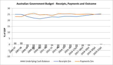
A frequent debate is whether Australia’s budget situation is caused by a problem with expenditure, revenue, or both. Looking at the summary of budget results in Figure 3, it can be seen that Commonwealth Government expenditure, has remained relatively static at around 25% of GDP

It can be seen that in 2007-08, coinciding with the Global Financial Crisis, expenditure rose and revenue fell in GDP terms. While

Figure 6: Budget Outcomes (GDP Share) 2006-07 to 2020-21


Receipts

Expenditure

2006-07

25.1

23.3

2007-08

25

23.1

2008-09

23.2

25.1

2009-10

21.9

26

2010-11

21.4

24.5

2011-12

22.1

24.9

2012-13

23

24

2013-14

22.7

25.6

2014-15

23.4

25.5

2015-16

23.4

25.6

2016-17(e)

23.2

25.1

2017-18(e)

23.8

25.2

2018-19(e)

24.4

25.4

2019-20(p)

25.1

25

2020-21(p)

25.4

25

Election Timing

With a federal election due in 2019, if the forecasts described above play out, the government will either have delivered or be preparing a budget with a small deficit.

While this has obvious benefits in terms of evidence of an improving fiscal situation, this small surplus will mean that the government will have limited scope to engage in election promises in the short term.

After reducing government receipts (in GDP terms) in 2016-17, it will have increase revenue in the previous two years – every budget since the last election. If the budget has been delivered, there will have been a reduction in expenditure in GDP terms from 25.4% to 25%.

However, the Government is expecting to be experiencing stronger economic growth than any time since 2014-15, lower unemployment, and inflation within the RBA comfort zone, albeit slightly higher than in previous years.

Given that the economic forecasts for 2018-19 and 2019-20 are associated with significant uncertainty, and that the 2019-20 budget is likely to involve reductions in expenditure and increases in revenue, it is likely that the government will call an election before delivering the budget in May

The Laffer Curve: Now Who’s Laffering

The Laffer Curve became popular in the 1980s as an argument for reducing tax rates.

The Laffer Curve, as shown below, is the illustration of the idea that it may be possible to increase tax revenue by reducing the tax rate. This concept is tantalising for politicians electorally popular tax cuts while not requiring the accompanying reduction in government receipts.

The view of the Laffer curve tends to be strongly influenced by political persuasion. A left-wing conceptualisation of the Laffer curve assumes that these effects only take effect at high taxation rates as shown in the left-hand chart in figure 1. A right-wing view of the Laffer curve shows that even relatively low rates of taxation can be reduced to increase tax revenue.

Figure 1: The Laffer Curve – two points of view


The Laffer Curve is often used to draw macroeconomic conclusions – to support statements such as “reducing taxes may actually increase revenue”. However, unless all taxes are assumed to be on the same activity, or completely unrelated to each other, there will be interplay between tax revenues from the various sources, which will in turn lead to a less smooth curve than that illustrated above, possibly featuring discontinuities, local solutions which differ from the global optimum will arise. In a Federal situation, where there may not be cooperation between the governments taxing, the situation will become akin to game theory – where a tax rate needs to be selected given other governments tax rates.

There are several important points about the Laffer curve:

  1. In essence, it is not an economic theory. It is an economic identity, which falls directly out of the maths. If we assume that tax revenue is zero if the amount of activity being taxed is zero and that at some sufficiently high level of taxation all taxpayers will be forced out of participation, tax revenue at that point will also be zero. Between these two points, there will be (at least) one rate of tax which is associated with the highest revenue. Any economic model with a tax that can be avoided can have a Laffer curve derived.
  2. The maximum point of the Laffer Curve is probably not as important as the slope. The government is unlikely to seek to maximise its revenue as its primary objective – even if it involves lower tax rates, there is considerable anecdotal evidence that there is a preference for lower government revenue as a proportion of GDP. This redefines the interpretation of the above curves as being the left-wing belief that collecting additional revenue will require significant increases in the tax rate, while right wing governments would tend to see that smaller increases in the tax rate will be sufficient to collect required revenue. (This is, in turn, assuming that the tax rate is operating on the left-hand side of the Laffer Curve, where the tax rate is lower for a given level of revenue, and minimising the distortion introduced into the economy associated with the tax.
  3. The tax rate, which is traditionally assumed to force revenue to zero at 100% may not do so. In the context of consumption taxes or similar -where the tax is added to the price, a 100% percent tax rate does not imply zero demand. Essentially, if a price is doubled by a tax, consumption will not necessarily stop. An income or profit tax levied at 100%, may not completely eliminate that activity.
  4. The Laffer curve does not make sense in the case of non-distortionary taxes – i.e. taxes which don’t change behaviour. A profit maximising firm will not change its output if the tax is a constant percentage of profit. Therefore, the tax rate which will maximise government revenue will be marginally below 100%. This is obviously of limited suitability as a policy prescription.
  5. The slope of the curve, which is asymmetric in both the left-wing and right-wing cases. If a policymaker, recognising the uncertainty surrounding any estimate of the Laffer curve, takes a probabilistic view of the Laffer curve, where the tax rate is chosen on the basis of maximising expected revenue, then some interesting results will ensue. A left-wing policy maker, recognising the potential for a rapid decrease in tax revenue if the tax rate is too high is likely select a tax rate which is below that which will maximise revenue – a move towards the right-wing policy makers preferred outcome. Similarly, a right-wing policy maker facing uncertainty is likely to select a higher tax rate given the risks associated with overshooting the optimal tax rate.


The Laffer Curve can be easily derived.

If we assume costless production, a tax of $t per unit a demand curve which relates price, p, to quantity sold, q, and parameters a and b in the form

Profit of the firm will be:

In order to maximise profit, the firm will differentiate the profit function, set the derivate to zero and solve for q, which we will denote q*.

This allows derivation of the Laffer curve, with R being government revenue:

Yielding the revenue maximising tax of:

Which has a relationship to the parameters of the demand curve, but no connection to the price of the good.

If we convert this to a percentage tax:


Which is a truly remarkable result. It says that if we have a linear demand curve and zero demand curves, the revenue-maximising tax rate is 66% of the product price.

While these assumptions are relatively strong, they are indicative of some interesting results which are hidden in the Laffer Curve.

It also indicates a relatively high rate of tax – which is more in line with the left wing view of the curve.

Further investigation to come…


Design Principals When Building an Excel Model

Simplicity

The most important feature your model needs to have is simplicity. No matter how complex the problem, the structure of a spreadsheet is perfect for that problem to be broken down into components, solved at this level, and these solutions to be rolled together into an answer to the problem.

The practical implementation of this means:

  • Keep your formulae short. Spread more complicated calculations over a number of cells.
  • Use worksheets to break your work into sections. A financial model might have a separate tab for revenue calculations and expense calculations. As complexity increases, these calculations may be further divided.
  • If you are performing a calculation using values from a different sheet, bring those values into the current sheet, and then perform the calculation. That not only reduces the size of the formula, but makes it much easier to see what values are being used in the calculation.

Complications make your model harder to audit, maintain and understand.


Unique cells

One of the most important design principals in Excel is avoiding unique cells. These are cells which we can’t predict the contents of based on the information surrounding them. These cells should be avoided at best, or highlighted and explained at a minimum. This section will describe how they arise and how to manage them.

  • A transition from raw data to a formula.
  • A formula changes along a row or down a column.
  • Deviation from the purpose of the sheet.

Introducing Formula

A spreadsheet contains a row of data. However, at some point it changes from a hard coded value to a formula – perhaps repeating the last data point, calculates an average, or applies a growth rate. The reason this has occurred is likely that the model required data beyond the inputs available, necessitating an assumption about what happens next. For example, exchange rate forecasts span five years, and after that we apply that last forecast for the remainder of your model.

This is relatively common, and should be managed by highlighting the cell where the formula is introduced and including commentary about the model.

Changing Formula

This is typically a sign of a model in distress. A row/column contains a complicated formula – think nested =IF() statements. It has been modified over many periods to overcome the occasional quirk with the data. Under time pressure, we add another condition until we get that cell right. We continue this process as circumstances change.

The solution to this situation is to review the logic of your formula. Consider simplifying and spreading over a number of columns or rows. Are the other ways to approach the problem which a more transparent and auditable? Investigate these issues.

Changing Sheet Design

Almost all of the data on a sheet is time series. However, a few assumptions are for all periods. These assumptions are in the column which is meant to hold first year data. This means that a user who is examining these cells may be confused – do they only apply to year 1? If so, what happens in other years?

This situation arises during development of the model, where we are inserting assumptions, and it may be easier to group assumptions by topic – put everything associated with revenue on the same sheet. However, now we have a fully functioning model, it is time to create the necessary sheets and adjust the layout to reflect best practice modelling.

Incorrect numbers

A financial model aims to calculate an after tax return, and is labelled appropriately. However, due to an error in the formula, it actually calculates a pre-tax return. Or a user mistakenly entered a pre-tax number where post tax is required.

These cases are more difficult to detect than the above examples, which can be identified by visual inspection alone. In the case of user input, it may be almost impossible to detect without reviewing the source data and a good understanding of the business being modelled.

The solution in this case is the use of alerts, or built-in sense checks. For example, an alert may be raised where the post-tax return is higher than the pre-tax return.

Conclusion

This will hopefully give you some ideas for how to develop stronger models which can continue to be useful into the future.


Deliberate errors and model reviews

An important part of the development of a model is a review of the model – either by a colleague or a more formal external review.

An important aspect of this is incorporating deliberate errors in the model. These errors are recorded, and the model version with these errors is clearly marked as such and not used for analysis. This provides two key benefits:

  • By finding all of the deliberate errors, the reviewer will demonstrate that they have carried out the review thoroughly and that it is likely that the genuine errors are discovered; and
  • Selecting the deliberate errors in the model provides an opportunity for reflection on model logic and assumptions.

The deliberate errors selected should reflect those which are likely to be included in the development model:

  • Formatting – that all cells comply with formatting rules.
  • Formula errors – referring to incorrect cells or ranges, using inappropriate calculations (e.g. adding rather than multiplying).
  • Logic errors – where the formula does not calculate the desired figure – for example multiplying by the incorrect currency.
  • Deviations from best practice – including hard coded values, repeating inputs etc.

Finally, before you submit a model for review, do a thorough review of the model yourself.

EconomicsLAB provides model review services. If you would like to discuss this, or any other issues in analytics and economics, please contact adam@economicslab.com.au.


Named ranges in Excel – a good idea?


I am in two minds about named ranges.

Named ranges allow a formula to capture the logic of the calculation in an easy to understand way – illustrating the developers thought process and assumptions.

=Cost_Price*(1+MarkUp)

While this helps logic reviews, it does make it more difficult to review accuracy. When using named ranges, reviewers need to both (i) identify which cells are being referred to by the named ranges, and (ii) ensure they contain the appropriate value. This introduces an additional step in the review. Further complications can arise when ranges have similar names, ranges appearing in multiple worksheets.

The biggest difficulty with named ranges, however, is the vast number of redundant ranges which seem to accumulate. Incrementing versions of the model over time or the course of development, copying between workbooks, all seem to cause this problem. The impact of this is slower performance, increased file size, and decreased stability of the model.

EconomicsLAB’s First Aid Kit is an Excel add-in which addresses this issue, and other common Excel problems. If you would like further information or would like us to tailor a solution to your needs, please contact adam@economicslab.com.au.


Excel and Dimensionality

One the biggest lessons I have learnt in Excel is that it is a two dimensional tool – rows and columns. At a stretch, we can do three (rows, colums and sheets). However, a lot of the time, we call on it to operate in a more complicated scenarios.

I was once tasked with reviewing a model which calculated the balances of four accounts for around fifty sites. In the short-term, the calculations were done on a six monthly basis. That moved to annual later in the period.

The resulting model was complicated, and very hard to extend. There were errors in the output, but it was difficult to find and correct them. The sites were listed along the rows, with the account balances and dates listed in the columns, with some initial assumptions in the early columns. This had several problems. It was very hard to follow the logic of the model – formula for each period referred to a mixture of the assumptions and previous period. When the model switched from sig monthly to annual, the formulae were inconsistent.

Rather than remedying the model, it was easier to redevelop the model. A better structure was a table with the assumptions on a separate sheet. The calculation/output sheet looked up these results, using a drop down box to select the site. Account balances ran across the columns, with the periods running down the side. Because the layout and calculations were now much simpler, we moved to a monthly basis of calculation, with sums to provide six monthly/annual totals. Charts became easy to include, and were great for finding errors in the assumptions.

By removing one dimension, the result was a more user friendly, accurate, and extendable model.

If you require any analysis of spreadsheets, including model reviews, development of add-ins or macros, contact adam@economicslab.com.au.

Welcome

Welcome to EconomicsLAB. We provide financial analysis, modelling and development of Microsoft Excel solutions for businesses.

More content is coming soon, together with some exciting products.